Ground Track Generator

This small project was to write a script that robustly plots ground tracks for a given set of orbital elements. The arguments to the function ground_track.m are the set of (constant) orbital elements $\{a,e,i,\omega,\Omega\}$ , a starting true anomaly $\theta_0$ , and the number of periods to plot.

The function currently assumes constant $a,e,i$ , but does incorporate earth $J_2$ effects which have the effect of creating nonzero $\dot{\omega}$ and $\dot{\Omega}$ . In the future I’d like to incorporate various other disturbances and perturbations such as atmospheric drag and perhaps solar pressure for higher orbits.

The Solver

As mentioned, the solver incorporates $J_2$ effects, however these are easy to deal with since the derivatives of $\omega$ and $\Omega$ are constant. So the integration is very simple to carry out:

$\begin{align} \Omega(t) &= \Omega_0 + \dot\Omega \, \delta t \\ \omega(t) &= \omega_0 + \dot\omega \, \delta t \end{align}$

From here use Kepler’s method to solve for the true anomaly $\theta$ at each desired timestep. Then it’s a whole lot of coordinate transformations to finally arrive at the ground track longitude and lattitude of the satellite as observed from a rotating earth.

Some Results

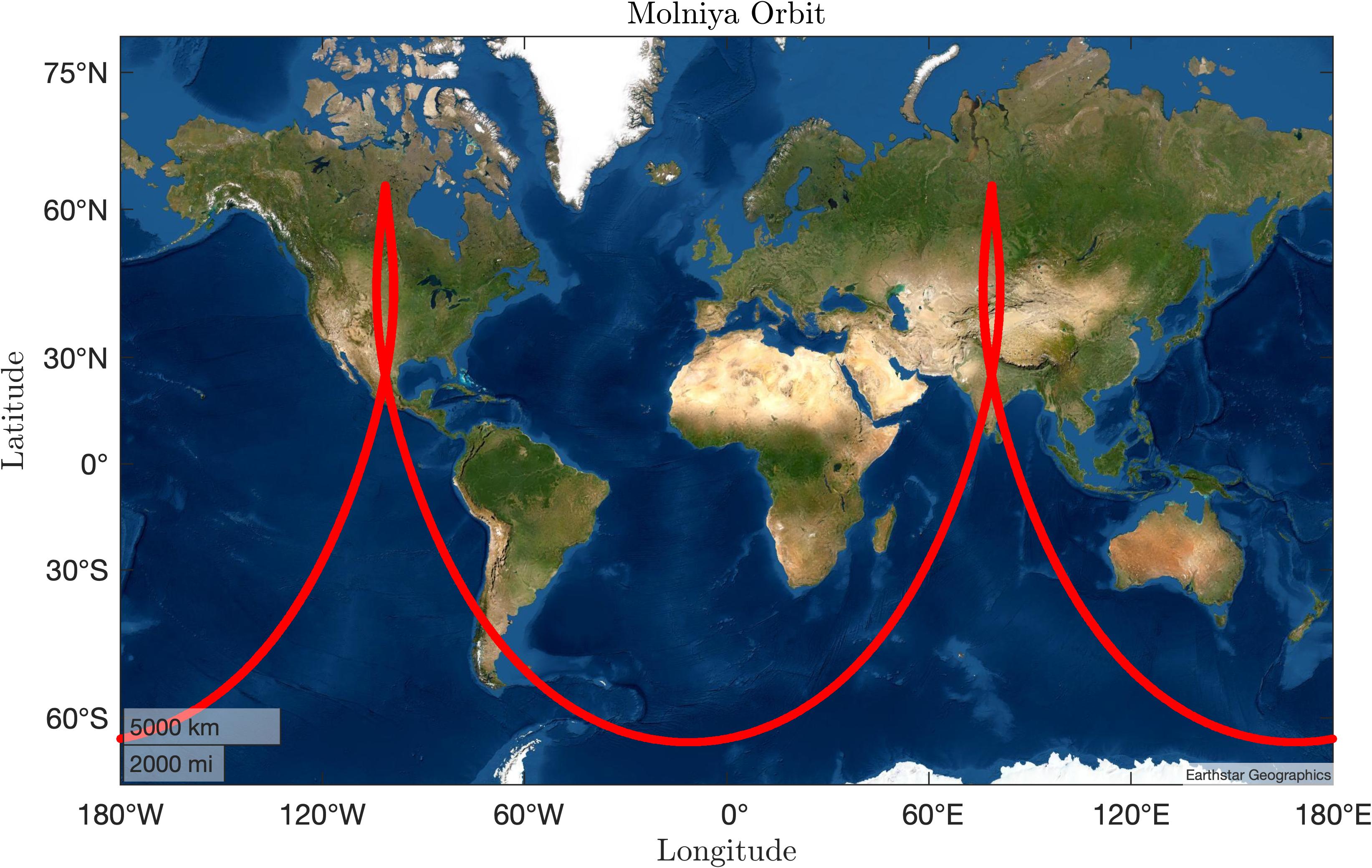
Here are some results! Not too much to say other than the plots look as we would expect them to. Shown below is a Molniya Orbit, made popular by Soviet spy satellites.

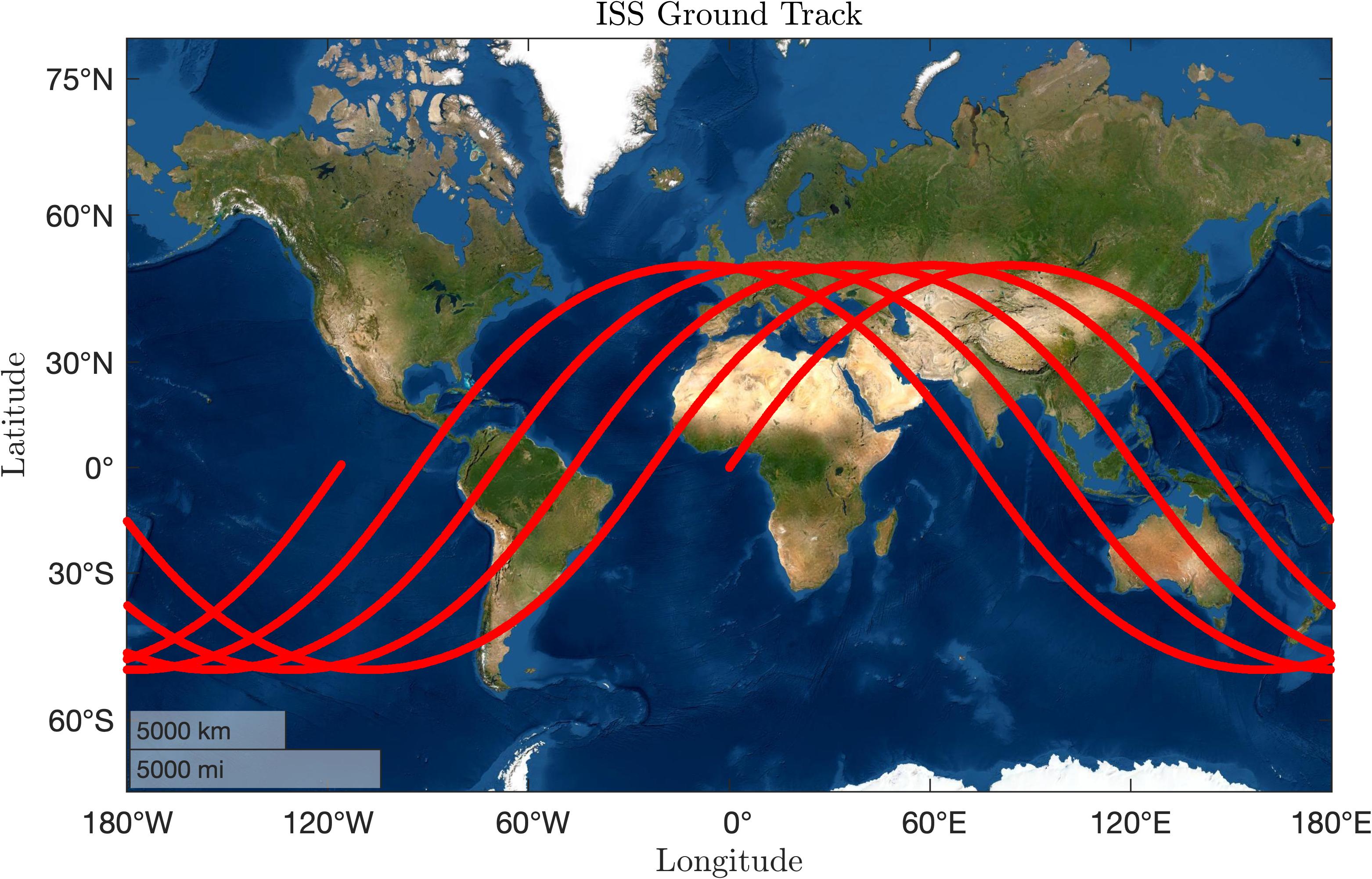
Here’s an orbit we’re all familiar with, which is the ISS’s orbit. It’s plotted here for 5 periods.

Future Work

There are a number of things I think would be cool to implement into this project.

The first thing I want to do is include support for multiple satellites at once. This would allow for visualizing complex constellations and showing constellation coverage of the surface of Earth.
Also it would be fun to implement a high-fidelity orbit for the ISS and query the current time when the user runs the ground track function. This would allow for showing the current position of the ISS in the sky.
And as mentioned, I want to incorporate a larger variety of disturbances and perturbations. Implementing drag would be especially interesting for LEO satellites.